


The complete 64-node map is reproduced below as a reading edition. Open the original interactive map to expand and collapse its branches.
Interactive map · AI Memory, Step by Step
The AI Memory Hierarchy
One argument, from the physics of storing a single bit to the question of which part of the semiconductor value chain is paid when a particular constraint binds. Open any node to read it.
Independent research by Memory Capex As of 14 September 2026 64 nodes · three nested levels + root Companion to the three-part series
Part 1 — The Physics and Economics of Memory
Part 2 — What AI Actually Does to Memory
Part 3 — Where the Hierarchy Is Going
Tap or click any node to open its explanation; tap or click again to close it. Every node sits below the node it depends on.
Root — the argument Level 1 — the nine branches Level 2 — components of a branch Level 3 — detail within a component
Memory Hierarchy for AI 9 sub-nodes
This map is a single argument, not a glossary. It runs from the physics of storing one bit to the question of which part of the semiconductor value chain is paid when a particular constraint binds. Every branch is a step in that argument, and each depends on the ones above it.
The organising claim is that AI memory is not one market or one technology. It is a hierarchy assembled from incompatible compromises in speed, capacity, persistence, energy and cost. Because no device maximises all of them, systems are built as layers, and the layer that limits a given workload decides where money and engineering effort go.
The first branches establish what memory is and what AI workloads do to it. The middle branches explain why HBM had to be invented, how data is tiered across the hierarchy, and which interconnects and emerging tiers are reshaping it. The final branch translates all of that into exposure.
Open any node for its explanation. Quantitative claims follow the same primary-source register used in the linked three-part series; each node links back to the relevant sourced section.
Read this in full → Part 1 — The Physics and Economics of Memory
Physics and Economics 3 sub-nodes
Before any AI-specific reasoning, memory obeys a physical and economic logic that has nothing to do with machine learning. A processor cannot operate on data that is not in front of it, and getting data in front of it costs time, energy and silicon area.
That cost is not a single number. It splits into several properties that trade against one another, and the trade-offs are not soft preferences — they are rooted in cell structure, interface width, physical distance and manufacturing economics. A design that maximises one property structurally sacrifices another.
The consequence, which the rest of the map depends on, is that a memory system is a portfolio decision rather than a component choice. Systems buy several technologies at once and place each where its particular compromise is least damaging.
This is also why the memory industry does not converge on a single product. Different customers weight the axes differently, so several distinct businesses with different cost structures and capital intensity can coexist indefinitely.
Read this in full → Part 1 — The Physics and Economics of Memory
Data Movement Machine
The useful first model of a computing system is a loop: load, compute, store, move, repeat. Arithmetic receives most of the attention because it is where the visible work happens, but the other three stages determine whether the arithmetic hardware has anything to do.
Framing the machine this way changes what counts as a bottleneck. A processor that is idle because its operands have not arrived is not short of compute; it is short of delivery. The economic implication is that spending on arithmetic capability has a ceiling set by the data path feeding it.
This is the conceptual shift that makes the rest of the hierarchy legible: the processor is not an isolated engine, it is one component of a system whose job is to place the right bytes close enough at the right moment.

Read this in full → Part 1 — The Physics and Economics of Memory
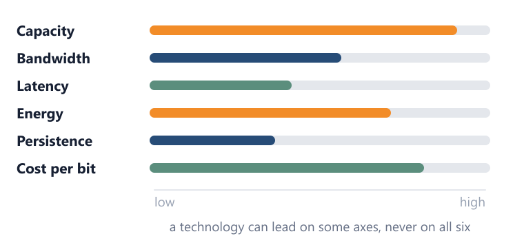
Six Trade-off Dimensions 6 sub-nodes
Saying a memory technology is “better” is incomplete until you say better on which axis. Six independent properties matter, they interact, and none substitutes for another.
The important structural point is that improving one axis usually costs another through a physical mechanism, not through vendor choice. Making a cell smaller raises density and lowers cost per bit, but tightens electrical margins. Widening an interface raises bandwidth, but consumes package area and power. Moving memory closer to compute lowers latency, but competes for the most expensive silicon real estate on the system.
Because the axes are independent, two customers can both be buying “more memory” while solving entirely different problems and creating entirely different demand for silicon, packaging and equipment. Confusing the axes is the single most common analytical error in reading the memory market.
Read this in full → Part 1 — The Physics and Economics of Memory
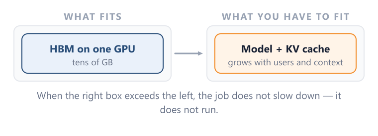
Capacity
How much information can be held at all. Capacity is a gating condition: a system can be excellent on every other axis and still fail if the working set does not fit.
Its economic signature is demand for bits — more die area, more wafers, more packages. It says nothing about how quickly those bits can reach compute.
Read this in full → Part 1 — The Physics and Economics of Memory
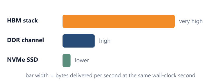
Bandwidth
How much information can cross the memory interface per unit time. Bandwidth is a throughput property of the pipe, not of the reservoir behind it.
Its economic signature is interface width, signalling rate and packaging complexity rather than raw bit count. This is why bandwidth-driven demand and capacity-driven demand can move different suppliers in different directions at the same time.
Read this in full → Part 1 — The Physics and Economics of Memory
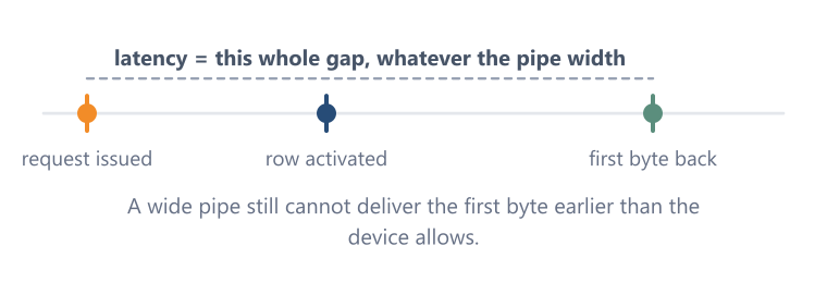
Latency
The delay before a single requested access begins to deliver useful data. A system can have very high aggregate throughput and still impose meaningful waiting time on an individual request, which is why latency and bandwidth are not interchangeable measures.
Read this in full → Part 1 — The Physics and Economics of Memory
Energy
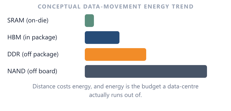
Reading, writing and physically moving information all consume power, and the farther data travels and the more interfaces it crosses, the larger that share becomes. The relevant metric is not the power rating of a chip but the energy required to deliver useful data where computation needs it.
Read this in full → Part 1 — The Physics and Economics of Memory
Persistence
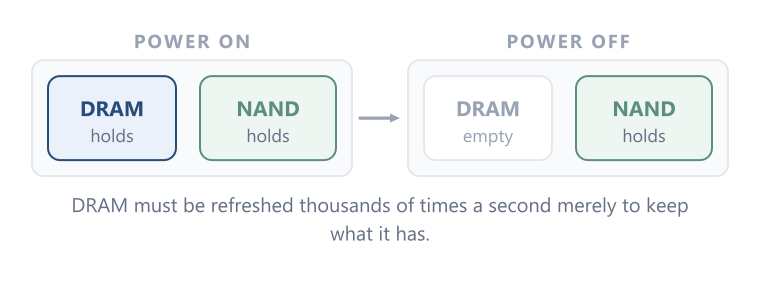
Whether stored information survives loss of power. SRAM and DRAM are volatile and depend on continued power; NAND flash is non-volatile, which is what makes it suitable for storage rather than working memory.
Read this in full → Part 1 — The Physics and Economics of Memory
Cost per bit
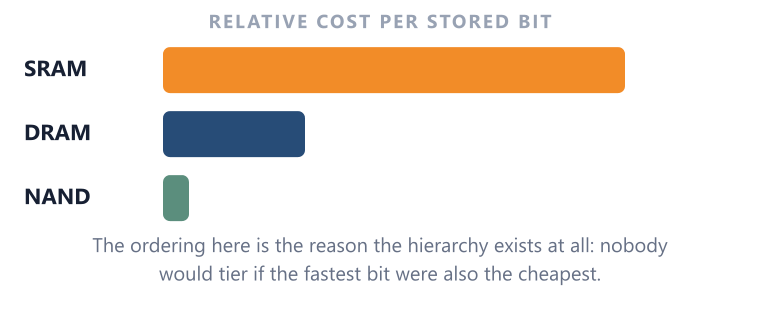
The economic cost of providing a given quantity of stored information. It incorporates far more than chip price: silicon area, process complexity, yield, packaging, controllers, power and system integration all feed into it.
Because these inputs differ sharply by technology, cost per bit is the axis that ultimately forces the hierarchy to exist rather than collapsing into one universal memory.
Read this in full → Part 1 — The Physics and Economics of Memory
Incompatible Optimization Goals
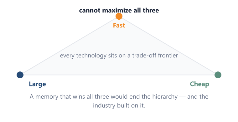
The hierarchy is not a historical accident or an engineering convenience. It is the system-level response to the fact that the six axes cannot be maximised together.
Moving up the hierarchy improves proximity and access performance while raising the economic cost of every stored bit. Moving down allows far larger capacity at lower cost but with slower access. No single tier can economically replace the others, which is why the structure has survived every generation of memory technology so far.
For an analyst this is the reason the sector has durable, distinct sub-markets rather than one commodity curve.
Read this in full → Part 1 — The Physics and Economics of Memory
Storage Technologies 3 sub-nodes
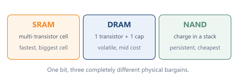
Beneath the product names sit three genuinely different physical methods of representing a bit, and those methods are what generate the trade-offs above.
The distinction matters commercially because it separates the industry into businesses with different capital intensity, different process roadmaps and different cycle behaviour. It also settles a confusion that recurs constantly in market commentary: DDR and HBM are not competing memory families, they are two architectures built on the same underlying DRAM technology, while NAND belongs to a different family entirely.
Read this in full → Part 1 — The Physics and Economics of Memory
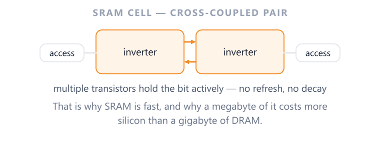
SRAM
Stores state in a circuit of multiple transistors. As long as power is present the circuit holds its value without the periodic refresh DRAM requires.
The trade-off is area: an SRAM cell consumes substantially more silicon per bit than a DRAM cell, so large capacities are prohibitively expensive. That confines SRAM to small, speed-critical structures on the processor die, and makes it a consumer of scarce logic-die area rather than a separate memory market.
Read this in full → Part 1 — The Physics and Economics of Memory
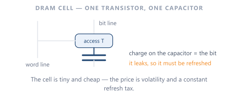
DRAM
Uses a conceptually simple cell built around one transistor and one capacitor. The capacitor holds charge and the transistor controls access; because the charge leaks, the contents must be refreshed periodically, which makes DRAM volatile.
That compact cell is what allows far higher density than SRAM. Samsung lists DDR, LPDDR, GDDR and HBM together as DRAM product families — the clearest public confirmation that HBM is an unusually sophisticated form of DRAM, not a new memory physics.
Read this in full → Part 1 — The Physics and Economics of Memory
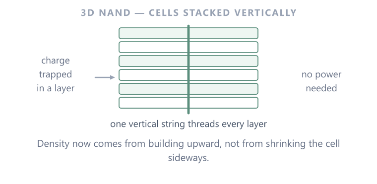
NAND
Retains information by trapping charge in a storage structure, so data persists after power is removed. Cells are arranged vertically to raise density.
This makes NAND the economic base of the hierarchy — large persistent capacity at the lowest cost per bit — rather than a substitute for DRAM. A finished SSD is also more than flash: controller, firmware, interface and error correction are a meaningful part of the product and of the margin.
Read this in full → Part 1 — The Physics and Economics of Memory
AI Workload Occupants 5 sub-nodes
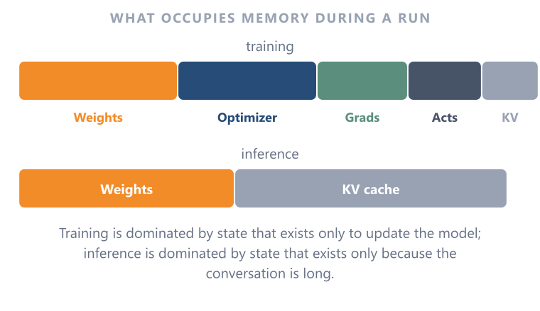
Once the hierarchy exists, the question becomes what actually occupies it. An AI workload does not store one undifferentiated blob; it stores several kinds of state with different sizes, lifetimes and growth drivers.
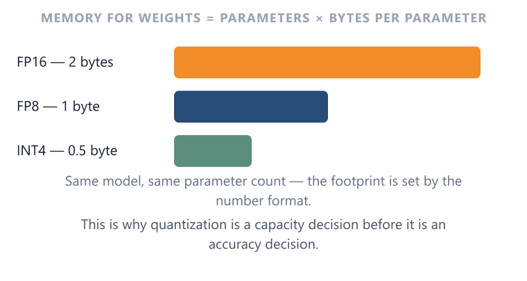
Weight memory is the only component that follows directly from model size, and it is arithmetic: parameter count multiplied by bytes per parameter, where the byte width is set by the numeric format. Everything else scales with how the model is being used rather than how large it is.
This is why parameter count is a weak predictor of memory demand. Two services running an identical model can have radically different footprints depending on training versus serving, context length, batch size and concurrency — and those differences translate into different purchases of capacity versus bandwidth.
Read this in full → Part 2 — What AI Actually Does to Memory
Weights
The learned parameter values. Their memory cost is the one quantity that can be estimated from first principles: parameters multiplied by bytes per parameter.
Numeric format therefore acts as a direct multiplier on weight memory, which is what makes reduced precision such a powerful lever and why format support is a first-order hardware feature rather than a software detail.
Read this in full → Part 2 — What AI Actually Does to Memory
Activations
Intermediate results produced as data passes through the network. Some are transient; during training, forward-pass activations must be retained for the backward pass, which makes them a significant and batch-sensitive consumer of memory.
Read this in full → Part 2 — What AI Actually Does to Memory
Gradients
The error signals computed during the backward pass that indicate how each parameter should change. They exist only in training and are broadly proportional to parameter count.
Read this in full → Part 2 — What AI Actually Does to Memory
Optimizer State
Additional numerical state an optimiser maintains per parameter in order to compute updates. It is the least intuitive component and often the largest surprise in a training memory budget.
Microsoft’s original ZeRO analysis estimates roughly 16 bytes per parameter for a conventional mixed-precision Adam setup covering parameters, gradients and optimiser state together, before activation memory. Training is therefore state-heavy in a way inference never is. [P2:S9]
Read this in full → Part 2 — What AI Actually Does to Memory
KV Cache
The Key and Value tensors retained for previously processed tokens so that a transformer does not recompute all prior attention for every new token. It is the defining memory structure of inference at scale.
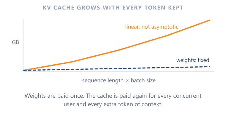
Its size is not set by model size alone. It grows with context length, layer count, attention design, numeric precision and — critically — the number of concurrent requests being served. A long-context, high-concurrency service and a short-prompt chatbot running the identical model occupy entirely different amounts of accelerator memory.
That variability is what makes KV cache an operational and economic problem rather than a fixed overhead. Capacity dedicated to cached context is capacity unavailable for weights or batch size, so serving economics become a question of how much context a provider can afford to keep resident.
It is also why memory management software became strategically important: allocation waste in a structure that changes size per request translates directly into wasted accelerator hours.
Read this in full → Part 2 — What AI Actually Does to Memory
Training vs. Inference Dynamics 3 sub-nodes
The same model stresses memory differently depending on what is being done with it, and the difference is not one of degree but of kind.
Training must hold model state, gradients and optimiser state simultaneously, plus retained activations, so it is dominated by the sheer volume of state. Inference discards gradients and optimiser state but introduces the problem of serving many users at once, where the binding resource is often the rate at which weights and cached context can be re-read.
This split is the mechanism that converts AI adoption into specific silicon demand. A world weighted toward training buys capacity to hold state; a world weighted toward large-scale serving buys bandwidth and proximity. Both are “AI memory demand” and they are not the same trade.
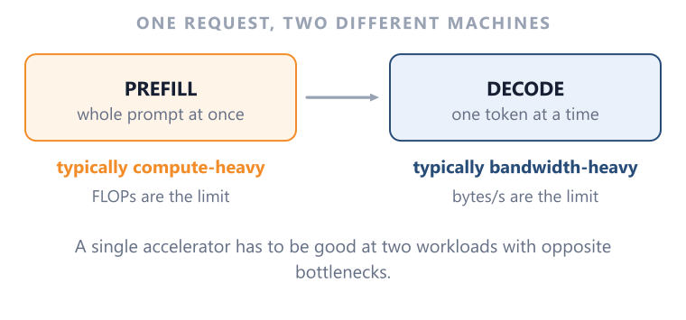
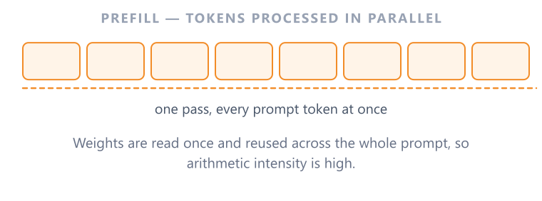
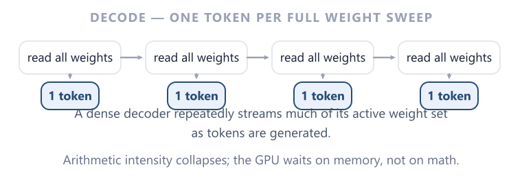
NVIDIA’s own framing of inference separates a compute-heavy prefill stage from a bandwidth-sensitive decode stage, which is the technical basis for treating the two phases as distinct workloads rather than one.
Read this in full → Part 2 — What AI Actually Does to Memory
Training: state-heavy
A training step runs a forward pass, computes error, runs a backward pass and updates parameters, holding weights, activations, gradients, optimiser state and communication buffers concurrently.
Because several of these scale with parameter count, training memory grows rapidly with model size and is typically solved by spreading state across many devices rather than by buying a larger single memory.
Read this in full → Part 2 — What AI Actually Does to Memory
Inference Phases 2 sub-nodes
Serving splits cleanly into two phases with opposite hardware profiles, which is why a single average utilisation figure describes neither well.
Understanding the split is what allows an analyst to predict whether growth in inference volume shows up as demand for arithmetic throughput or for memory bandwidth.
Read this in full → Part 2 — What AI Actually Does to Memory
Prefill
Processing the user’s prompt or context. Large matrix operations over many tokens at once make this phase typically compute-heavy.
Read this in full → Part 2 — What AI Actually Does to Memory
Decode
Generating tokens one at a time. Each step re-reads model parameters and the existing cached context while performing comparatively little arithmetic, so arithmetic intensity falls and memory bandwidth becomes the limiting resource.
Because most tokens a production service emits are decode tokens, this phase dominates the economics of large-scale serving.
Read this in full → Part 2 — What AI Actually Does to Memory
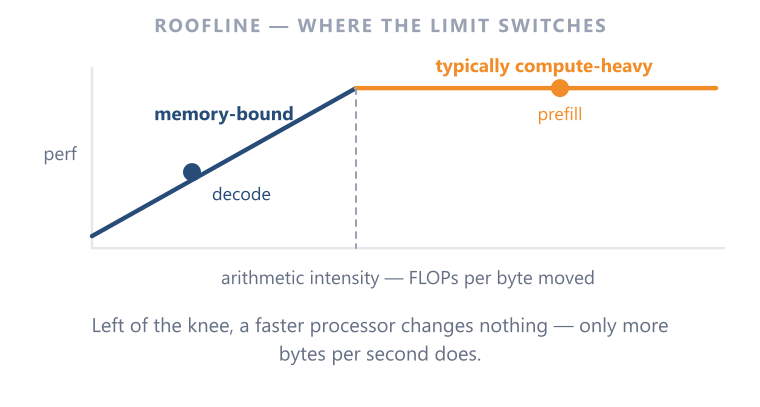
Arithmetic Intensity
The amount of computation performed per byte of data moved. It is the single number that decides whether a workload is limited by arithmetic or by delivery.
Roofline analysis formalises this: below a machine-specific threshold, adding compute changes nothing and only a wider or faster memory path helps. It is the bridge between the physics at the top of this map and the investment logic at the bottom.
Read this in full → Part 2 — What AI Actually Does to Memory
HBM and The Memory Wall 3 sub-nodes
This branch answers the question the rest of the hierarchy raises: why was a new, expensive class of DRAM necessary at all?
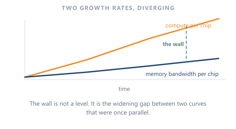
The answer is a divergence in growth rates. Across GPU generations, peak arithmetic throughput has risen faster than peak memory bandwidth. In one open-access comparison of peak dense FP16 tensor throughput against peak memory bandwidth, the endpoints move from 125 TFLOP/s and 0.9 TB/s to 2,250 TFLOP/s and 8 TB/s — roughly 18x against roughly 8.9x. These are theoretical peaks rather than achieved application performance, but the widening ratio is the point. [P2:S13]
HBM is the architectural response, and its significance for investors is that it is not a premium DRAM part. It is a co-designed subsystem spanning memory dies, logic and advanced packaging, which is why its economics pull in equipment, assembly and foundry players who never participated in commodity DRAM cycles.
Read this in full → Part 2 — What AI Actually Does to Memory
Memory Wall
The structural gap between how fast a processor can compute and how fast the memory system can deliver operands. It is a trend, not a state: each generation adds arithmetic faster than it adds delivery.
The practical consequence is diminishing returns on compute-only scaling, which is what forces architects to spend package area, power budget and cost on the memory subsystem instead.
Read this in full → Part 2 — What AI Actually Does to Memory
HBM Subsystem 4 sub-nodes
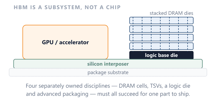
HBM does not make DRAM cells faster. It makes the connection between DRAM and compute dramatically wider and physically shorter, by stacking memory dies vertically and placing the stack immediately beside the accelerator on a shared package.
That reframing explains the cost. Building it requires known-good dies, wafer thinning, through-silicon via formation, precise bonding, an increasingly capable logic base die, advanced packaging and thermal management — and yields compound across those steps, so a defect anywhere in the stack discards good dies with it.
It also explains the supplier map. Value migrates from the DRAM cell alone toward deposition, planarisation and metrology equipment, bonding tools, interposer and packaging capacity. For an analyst, HBM is best read as a memory-logic-packaging system whose bottleneck can sit in any of the three.
Read this in full → Part 2 — What AI Actually Does to Memory
Stacked DRAM dies
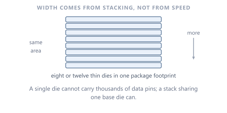
Multiple thinned DRAM dies placed vertically rather than spread across a board. Stacking is what converts a fixed footprint beside the accelerator into multiples of capacity, and it is the step that introduces compound yield risk.
Read this in full → Part 2 — What AI Actually Does to Memory
Through-Silicon Vias (TSVs)
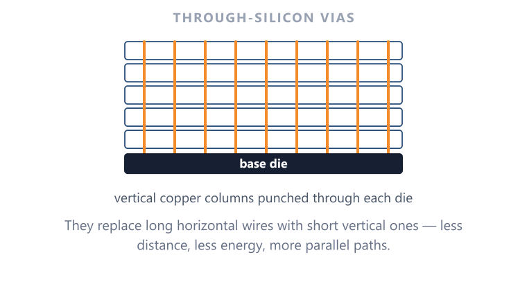
Vertical electrical connections punched through the silicon so signals travel between stacked dies over very short distances. They are what make a very wide interface physically possible, and their formation and alignment are among the most demanding process steps in the stack.
Read this in full → Part 2 — What AI Actually Does to Memory
Logic Base Die
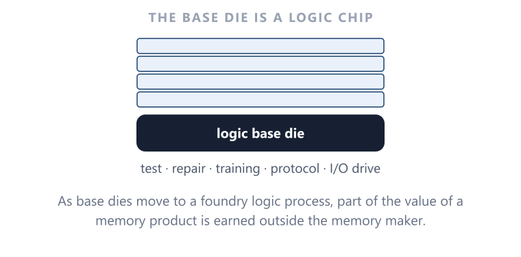
The die beneath the DRAM stack handles interface and control. In HBM4, the base die has become more logic-intensive: Samsung describes its commercial HBM4 base die as built on a 4nm logic process. [P2:S17]
That shift matters because it pulls a foundry logic process into what used to be a pure memory product, blurring the line between memory makers and logic manufacturing.
Read this in full → Part 2 — What AI Actually Does to Memory
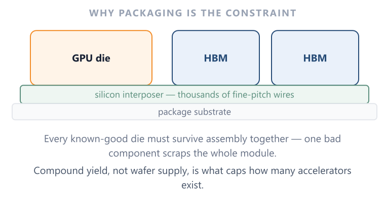
Advanced Interposer Packaging
The substrate that carries the thousands of short, dense connections between accelerator and memory stacks. Without it, a very wide interface cannot be routed at all.
Packaging capacity can therefore become a separate supply constraint on AI accelerators, even when DRAM or logic wafers are available.
Read this in full → Part 2 — What AI Actually Does to Memory
Roadmap
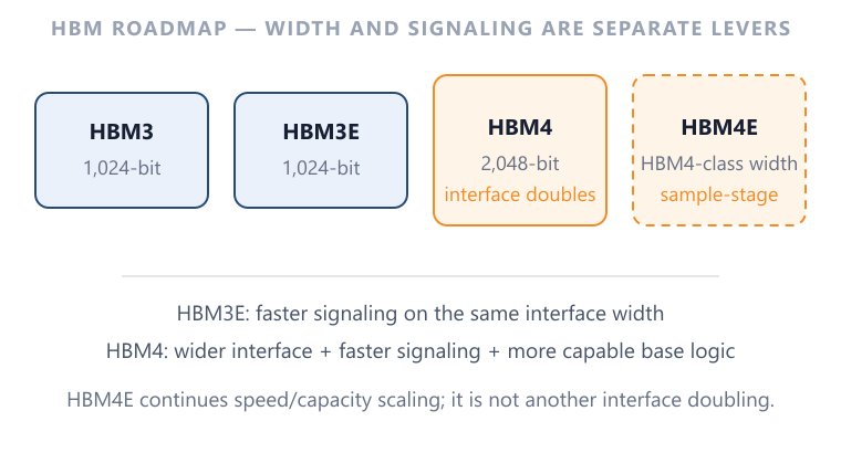
The generational path matters because it shows bandwidth being bought through three separate mechanisms: a wider interface, faster signalling, and tighter physical integration.
HBM4 widens the interface to 2,048 data signals against HBM3E’s 1,024. The JESD270-4 document itself is not publicly readable, so that figure is taken from JEDEC’s public announcement and corroborated independently by Micron and Samsung product statements. HBM4E continues the speed and capacity roadmap rather than doubling the interface again, and as of mid-2026 both Samsung and SK hynix describe it at sample stage. [P2:S17]
On the accelerator side the shipping reference points are H100 at 80GB and 3.35TB/s, H200 at 141GB and 4.8TB/s, and B200 at 180GB and up to 8TB/s. NVIDIA’s Rubin disclosure lists up to 288GB of HBM4 and up to 22TB/s, and NVIDIA stated on its 26 August 2026 earnings call that production shipments had begun. Those remain vendor-stated maxima rather than measured values for every configuration. [P2:S23]
Read together, capacity and bandwidth are scaling on separate tracks — which is precisely why they must be treated as separate demand drivers rather than one metric.
Read this in full → Part 2 — What AI Actually Does to Memory
Memory Tiering 4 sub-nodes
If HBM is so effective, why not put everything in it? Because it is scarce and expensive, and the scarcity is structural rather than cyclical — Micron has described HBM as consuming materially more silicon per bit than conventional DRAM.
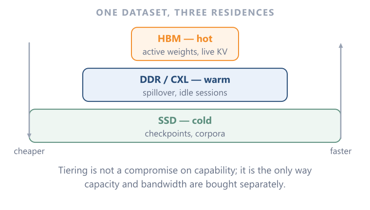
So systems tier. Data is placed according to how urgently and how often compute needs it, and it is promoted or evicted as that urgency changes. The scarce resource is not memory in general but fast memory close to compute.
This turns memory management into a scheduling and economic problem: at any moment, which byte has earned a place in the most expensive tier? Software that answers that question well converts directly into higher accelerator utilisation.
Read this in full → Part 2 — What AI Actually Does to Memory
Hot Data — HBM
The immediate working set: active weights and active cached context. Highest bandwidth, highest cost per byte, smallest pool. Anything resident here is displacing something else.
Read this in full → Part 2 — What AI Actually Does to Memory
Warm Data — DDR
System memory used for staging, host-side state and overflow that does not need immediate accelerator access. Larger and cheaper per byte, but a tier removed from compute.
Read this in full → Part 2 — What AI Actually Does to Memory
Cold Data — SSD
Persistent bulk: datasets, checkpoints, model files and retrieval corpora. Lowest cost per byte and effectively unbounded capacity, at the cost of being furthest from compute.
Read this in full → Part 2 — What AI Actually Does to Memory
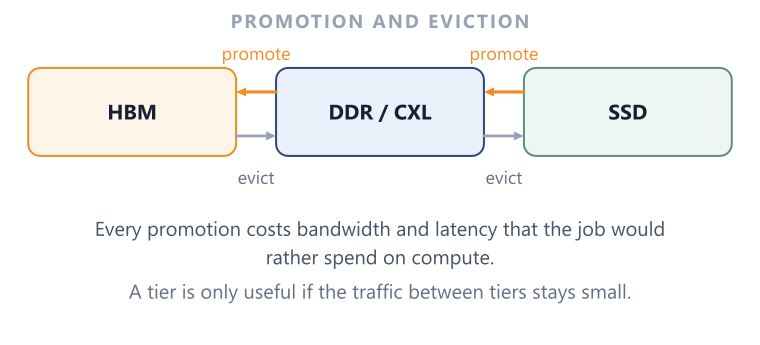
Data Movement (Promotion and Eviction)
Tiers are not static shelves. Data is promoted upward as it becomes active and evicted downward as it cools, and the traffic between tiers is itself a cost in time and energy.
Because every promotion consumes bandwidth that could have served compute, aggressive tiering can defeat itself. The quality of the placement policy, not the existence of tiers, is what determines whether the hierarchy helps.
Read this in full → Part 2 — What AI Actually Does to Memory
Emerging Interconnects and Tiers 3 sub-nodes
The established hierarchy has two visible gaps: capacity is locked to whichever host owns it, and the distance between expensive HBM and cheap NAND is very large. Three developments address those gaps from different directions.
None of them replaces a tier. CXL changes who owns capacity, direct storage paths shorten the route between persistent data and compute, and High Bandwidth Flash proposes an entirely new rung. Their common claim is that the hierarchy will gain structure rather than collapse.
For an analyst the useful discipline here is to separate what is standardised, what is commercially shipping, and what exists only as a specification target. The three children below sit at three different points on that scale.
Read this in full → Part 3 — Where the Hierarchy Is Going
CXL (Compute Express Link) 3 sub-nodes
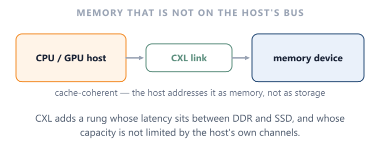
A cache-coherent interconnect that lets processors, accelerators and memory devices share an addressable memory space over a standard link. Switching, pooling and capacity-on-demand entered the standard with CXL 2.0. [P3:S28]
Its promise is allocation, not locality. Memory reached across a switch is still physically farther from compute than a stack sitting on the same package, so CXL does not reproduce HBM’s bandwidth or latency and is not a substitute for it. What it changes is that capacity no longer has to be permanently assigned to one host and stranded there.
The gap worth watching is between standardised capability and scaled deployment. Public demonstrations of expansion, pooling and disaggregated configurations exist, and commercial switching silicon exists, but how much pooled memory is actually running across large production AI fleets is hard to establish from public sources.
That uncertainty is itself the investable question: CXL connectivity is a small, concentrated exposure today whose size depends entirely on whether pooling becomes default architecture or stays a specialist deployment.
Read this in full → Part 3 — Where the Hierarchy Is Going
Memory Expansion
Adding addressable capacity to a single host beyond what its native memory channels allow. The simplest use of the standard and the least architecturally disruptive.

Read this in full → Part 3 — Where the Hierarchy Is Going
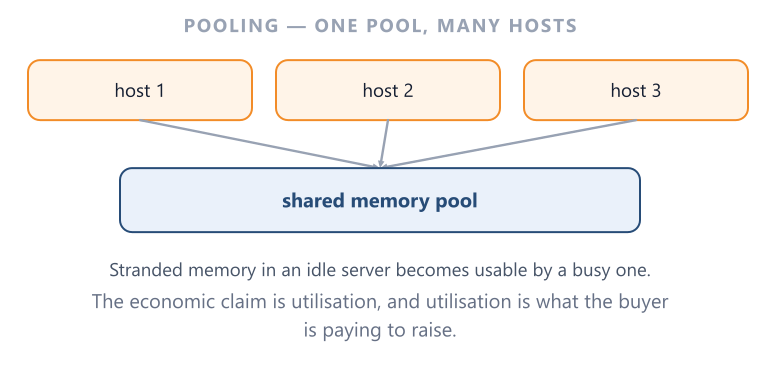
Memory Pooling
A shared pool that multiple hosts can draw from, so capacity idle on one machine can serve another. This is where the economic argument lives: stranded memory is paid for once and used partially.
Read this in full → Part 3 — Where the Hierarchy Is Going
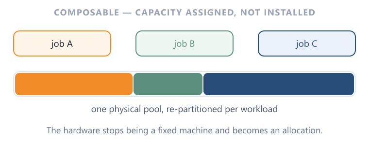
Composable Capacity
The end state in which memory is allocated to workloads on demand rather than being fixed to a chassis at purchase. Demonstrated publicly; not yet an established default.
Read this in full → Part 3 — Where the Hierarchy Is Going
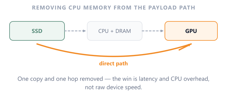
GPUDirect Storage
A direct transfer path between storage and accelerator memory, removing the host-memory bounce buffer from the payload route.
Two qualifications keep this honest. The payload still moves — nothing is free, and the bytes still cross a physical link. And the CPU still participates in control, even when it is no longer staging the data. What changes is the number of copies, not the existence of the transfer.
The reason it matters commercially is utilisation: at AI scale, storage throughput can decide how well extremely expensive accelerators stay busy, which is why storage performance now appears in AI benchmark suites alongside training throughput.
Read this in full → Part 3 — Where the Hierarchy Is Going
High Bandwidth Flash (HBF)
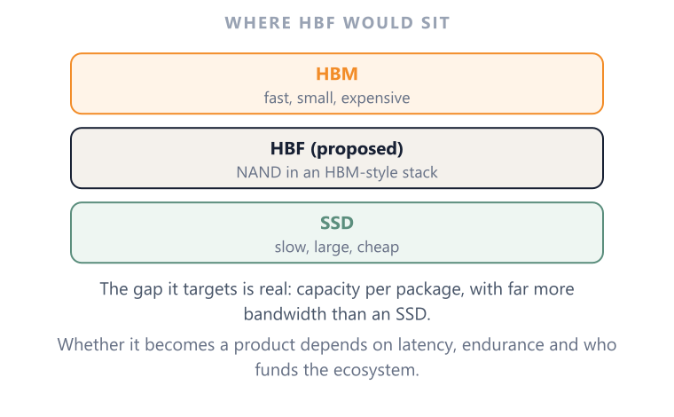
A proposed NAND-based tier sitting between HBM and conventional SSDs, aimed at the economic gap between very fast, very expensive memory and very cheap, comparatively slow storage.
Vendor-announced targets describe capacities up to 512 GB with bandwidth grades of roughly 0.4 to 3.0 TB/s over a UCIe interface. These are specification targets, not verified production performance. [P3:S41]
The verification limit should be stated plainly: the specification sits inside an Open Compute Project semi-private workstream and is not publicly readable, so the figures rest on the two proposing vendors’ announcements. HBF belongs on this map as evidence that the industry believes the hierarchy needs another rung — not as an established tier.
Read this in full → Part 3 — Where the Hierarchy Is Going
Scaling and Efficiency Levers 2 sub-nodes
Demand for memory is not set by hardware alone. Two very different levers change how much physical memory a given amount of useful work requires: making each device denser, and making software use a fixed device better.
They behave differently as investment signals. Density scaling is capital-intensive, supplier-visible and shows up as equipment and wafer demand. Software efficiency can improve utilization without installing more physical memory, but it can carry engineering, compute, communication or quality costs.
Treating only the first as “real” is the classic error in memory forecasting. Treating the second as a reason demand collapses is the opposite error.
Read this in full → Part 3 — Where the Hierarchy Is Going
NAND Density 2 sub-nodes
Density rises through two independent levers that can be pulled together or separately, which is why NAND has kept scaling long after planar shrink stopped being the mechanism.
The common cost of both levers is management: as cells hold more states and stacks grow taller, controller design, firmware and error correction absorb a growing share of the engineering and of the value of the finished drive.
Read this in full → Part 3 — Where the Hierarchy Is Going
Vertical Layer Count
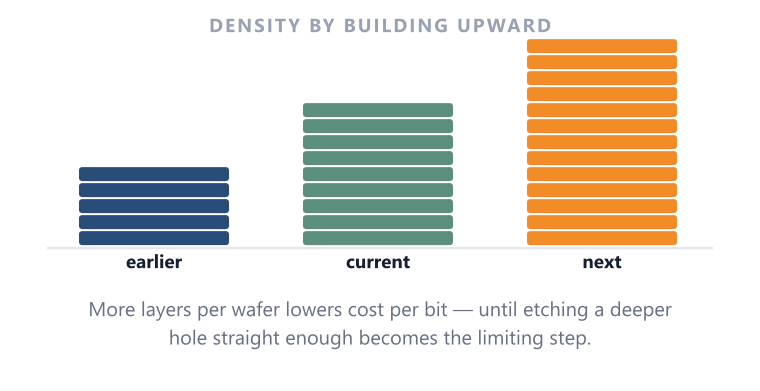
Building upward: more memory layers in the same footprint. Recent public examples describe 332-layer devices at sampling stage rather than broad volume production. [P3:S33]
Read this in full → Part 3 — Where the Hierarchy Is Going
Bits per Cell (SLC, MLC, TLC, QLC)
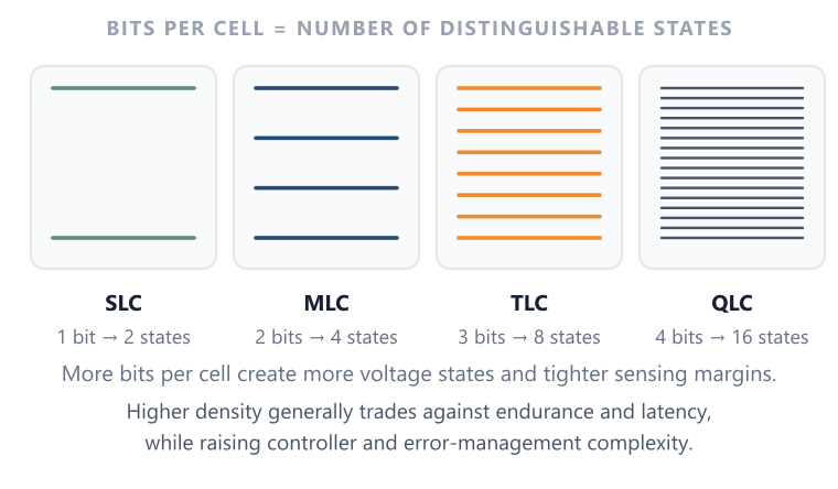
Encoding more information per cell — one, two, three or four bits. Each additional bit raises density and lowers cost per bit at the same layer count.
The price is narrower voltage margins, and therefore lower endurance and more demanding management. This is why QLC expands the addressable capacity market without simply replacing TLC.
Read this in full → Part 3 — Where the Hierarchy Is Going
Software Optimization 4 sub-nodes
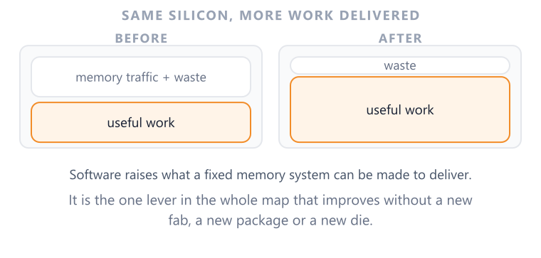
The physical memory block does not change size. What software changes is how much useful work fits inside it and how often data has to move.
Each of the four levers below buys something and pays for it somewhere else, and stating both halves is what separates analysis from marketing. None of them removes the underlying bandwidth and capacity constraints; they shift where the constraint binds.
The structural point for investors is that this is the one constraint in the whole map with no clean one-to-one listed-equity exposure. FlashAttention, vLLM and DeepSpeed originate substantially in research and open-source work. Efficiency can reduce hardware required per workload while also enabling more workloads, so its aggregate effect on hardware demand is not one-directional.
Read this in full → Part 3 — Where the Hierarchy Is Going
FlashAttention
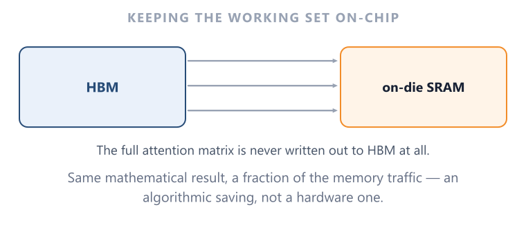
Reformulates attention as an I/O problem, restructuring the computation to reduce reads and writes between HBM and on-chip SRAM rather than to reduce arithmetic.
Benefit: fewer transfers for the same exact result. Cost: hardware-aware kernels and implementation complexity that must be re-tuned as architectures change.
Read this in full → Part 3 — Where the Hierarchy Is Going
PagedAttention
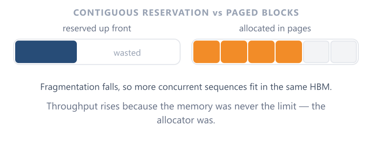
Manages the KV cache in fixed blocks, analogous to virtual-memory pages, so that a structure which grows and shrinks per request does not fragment the memory around it.
Benefit: far less waste and over-reservation, which raises serving throughput on unchanged hardware. Cost: block management and additional serving-layer logic.
Read this in full → Part 3 — Where the Hierarchy Is Going
ZeRO
Partitions optimiser state, gradients and eventually parameters across devices instead of replicating them on every one, directly attacking the state-heavy nature of training.
Benefit: models that would not fit become trainable. Cost: communication traffic and distributed coordination — the constraint moves from memory to interconnect.
Read this in full → Part 3 — Where the Hierarchy Is Going
Quantization and KV compression
Reducing numeric precision shrinks weights and sometimes cached state, making it the most direct lever on memory footprint.
The counterpoint deserves equal weight: the effect of compression is workload- and model-dependent, and aggressive KV-cache compression can degrade capabilities such as reasoning on some tasks while leaving others intact. Efficiency here is a trade, not a free gain.
Read this in full → Part 3 — Where the Hierarchy Is Going
Investment Value Chain 7 sub-nodes
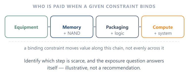
This is the only branch that names companies, and it does one job: it turns the technical map above into a question about exposure. The sequence is constraint, then supplying layer, then economics — never the reverse.
The reason the sequence matters is that “AI memory demand is rising” is not an investable statement. Rising demand for stored bits, rising demand for bytes per second, a shortage of packaging capacity and a shortage of DRAM wafers are four different conditions that pay four different sets of suppliers. Identifying which constraint is actually binding is the whole analytical exercise.
Two honest limits apply to everything below. First, this is an illustrative exposure map — not a recommendation, not exhaustive, and subject to change. Company names appear only as examples of product exposure to a named constraint, listed alphabetically within each layer, with no ordering that implies preference and no view on valuation.
Second, it ages faster than the rest of this map. Portfolios, packaging relationships and commercial exposure change even when the underlying hierarchy does not, so this branch should be re-checked whenever the series is revised. As of 14 September 2026.
Read this in full → Part 3 — Where the Hierarchy Is Going
Memory Manufacturers
Constraint served: HBM capacity and bandwidth, and DRAM supply generally.
Micron, Samsung and SK hynix each manufacture HBM alongside conventional DRAM families. Their exposure is unusual in that HBM ties a memory product to logic process and advanced packaging execution, so an operational problem in stacking or base-die supply can bind before cell capacity does.
Read this in full → Part 3 — Where the Hierarchy Is Going
NAND / Storage Suppliers
Constraint served: persistent capacity and the storage side of the AI data path.
Kioxia and SanDisk supply NAND flash and data-centre SSDs. This layer responds to dataset size, checkpoint volume, embeddings and retrieval corpora rather than to accelerator bandwidth, which is why it can move on a different rhythm from HBM.
Read this in full → Part 3 — Where the Hierarchy Is Going
Equipment Suppliers
Constraint served: DRAM wafer capacity and process intensity.
Applied Materials and ASML sell into the fabrication of advanced DRAM and, in Applied’s case, into advanced packaging as well. Exposure here is driven by capacity investment decisions rather than by bit shipments, so it leads or lags the memory makers depending on where the cycle sits.
Read this in full → Part 3 — Where the Hierarchy Is Going
Packaging and Logic
Constraint served: stacking yield and advanced packaging capacity.
Amkor, Applied Materials and TSMC participate in assembly, process equipment and heterogeneous integration. Advanced packaging becomes far more central to HBM economics than it is to conventional commodity DRAM modules.
Read this in full → Part 3 — Where the Hierarchy Is Going
Compute Integration
Constraint served: how much memory an accelerator can host and how tightly it is integrated.
Broadcom and NVIDIA design compute architectures whose memory subsystems are a defining specification. Their economics depend partly on keeping expensive arithmetic hardware supplied, which is why accelerator roadmaps now advertise memory capacity and bandwidth as headline features.
Read this in full → Part 3 — Where the Hierarchy Is Going
Connectivity
Constraint served: CXL switching and memory connectivity.
Marvell supplies commercial CXL switching silicon. This is a relatively concentrated connectivity exposure today, and its eventual size depends on how broadly pooled memory is deployed.
Read this in full → Part 3 — Where the Hierarchy Is Going
Software Efficiency — no clean listed exposure
Constraint served: nothing, in the supplier sense — and that is the finding.
Every other row on this map says a constraint binds, therefore spending flows to a layer. Software efficiency works the other way: it reduces the physical memory required for a given amount of useful work. Much of the progress originates in research and open-source projects such as FlashAttention, vLLM and DeepSpeed, so there is no clean one-to-one listed-equity exposure comparable with HBM manufacturing or NAND capacity.
Naming a single public company here would overstate the evidence. The honest reading is that this constraint can reduce hardware needed per workload while also enabling more total workloads; there is no clean one-to-one revenue exposure.
Read this in full → Part 3 — Where the Hierarchy Is Going
Source note: quantitative specifications and dated claims follow the primary-source registers in the three linked research parts; node links point back to the relevant sourced sections.
Illustrative exposure map — not a recommendation, not exhaustive, and subject to change. The Investment Value Chain branch names companies only as examples of product exposure to a named constraint, listed alphabetically within each layer, with no ordering that implies preference and no view on valuation.
MemoryCapex provides independent research and analysis for informational and educational purposes only. Nothing here constitutes investment advice, an investment recommendation, or an offer or solicitation to buy or sell any security.
The author holds, directly or indirectly, positions in substantially all of the publicly traded companies mentioned in this publication or series. Those positions may change without notice.
